Your enterprise RAG system treats every query the same way. A simple factual lookup about “Q4 revenue targets” goes through the exact same retrieval pipeline as a complex analytical question about “comparative market positioning across three quarters with regulatory context.” Both hit your vector database, both perform full semantic reranking, both wait for the same latency budget. One of them is being massively over-served; the other is being strangled.
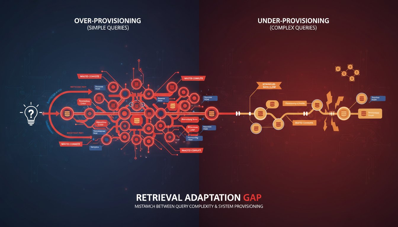
This is the Retrieval Adaptation Gap—and it’s draining millions in wasted compute cycles while simultaneously degrading user experience. Most enterprise RAG teams are aware of adaptive retrieval strategies in theory. They’ve read the papers on query-aware routing. They know that simple queries should take a different path than complex ones. But when deployment time arrives, they default to a uniform retrieval architecture because building query classification pipelines feels like “one more moving part” in an already complex system.
The problem is that this uniformity isn’t neutral—it’s expensive and ineffective. Simple queries get over-processed, burning through expensive vector operations and reranking passes they don’t need. Complex queries get under-served, processed through retrieval strategies designed for factual lookups instead of analytical reasoning. The result is a system that feels slow to users asking simple questions and unreliable to users asking nuanced ones.
But here’s what makes this gap particularly damaging in 2026: the tools and frameworks to implement adaptive retrieval have matured dramatically. We’re no longer building bespoke query classification systems from scratch. Enterprise teams now have access to proven architectural patterns, open-source orchestration frameworks, and cloud-native implementations that make dynamic retrieval strategy selection almost as straightforward as deploying a static pipeline—but with 40-60% efficiency gains.
The teams winning in enterprise AI right now aren’t just deploying RAG; they’re deploying intelligent RAG that recognizes query intent and routes accordingly. This post reveals exactly how to build that adaptive layer, the specific metrics that prove its ROI, and the implementation patterns that actually survive contact with production infrastructure.
The Hidden Cost Structure of Uniform Retrieval
Understanding why adaptive retrieval matters requires first understanding how much a uniform strategy actually costs.
Consider a typical enterprise RAG deployment at scale: 50,000 queries daily, mixed between simple factual lookups (“What’s our customer retention rate?”) and complex analytical questions (“Explain the relationship between customer retention and product feature adoption, considering seasonal patterns and competitor activity.”) Modern enterprise vector databases charge roughly $0.0001 per vector operation. A reranking pass with a cross-encoder model costs another $0.00015 per document scored.
In a uniform architecture, every query—regardless of complexity—retrieves the top-K candidates, typically 50-100 documents, and scores all of them. That’s roughly 50-100 vector operations and 50-100 reranking operations per query. At 50,000 daily queries, you’re performing 2.5-5 million vector operations and another 2.5-5 million reranking passes per day. The annual cost? Between $90,000 and $180,000 in processing alone—before considering infrastructure overhead, maintenance, and observability tooling.
Now add performance degradation. Simple queries don’t need deep semantic ranking; they need fast execution. Yet they’re waiting for full reranking passes designed for ambiguous queries. User-facing latency creeps up to 800ms-1.2 seconds. Complex queries, paradoxically, get worse results because they’re processed through shallow retrieval strategies. The system sacrifices accuracy on hard questions to maintain acceptable latency on easy ones.
Adaptive retrieval flips this model. Simple queries get routed to a lightweight path: maybe 10-15 candidate documents, no reranking, or lightweight keyword-based filtering. Processing cost drops to 10% of uniform cost. Latency drops to 100-150ms. Complex queries get the resources they actually need: deeper retrieval pools, multi-stage ranking, sometimes even graph-based context enrichment. The total system cost drops 40-60% while accuracy and latency both improve across query types.
How Query Classification Actually Works in Production
The theoretical promise of adaptive retrieval is straightforward. The production reality is messier—and more interesting.
Most enterprise RAG implementations use a three-tier query classification system, though the sophistication varies dramatically:
Tier 1: Intent Recognition — The system classifies queries into categories: factual lookup, analytical reasoning, temporal analysis, comparative analysis, or open-ended exploration. This isn’t learned from scratch; teams use either lightweight LLM-based classifiers (Claude Haiku or similar small models, which cost under $0.0001 per query) or rule-based systems (regex patterns, semantic similarity matching against exemplar queries).
Factual lookups like “What was Q3 revenue?” route immediately to a retrieval path optimized for exact matches. The system uses keyword search first, potentially skips semantic ranking entirely, and returns results in 50-100ms. Analytical queries like “Why did customer acquisition cost spike in July?” route to a multi-hop path that performs semantic search, then graph traversal to find related entities, then cross-reference with temporal data. This takes 300-500ms but returns semantically richer context.
Tier 2: Complexity Scoring — Within intent categories, the system scores query complexity. A simple factual query about a single metric versus a complex factual query about relationships between five metrics gets different treatment. Scoring happens through embeddings (compute the embedding, measure its semantic distance from known simple vs. complex exemplars) or through lightweight LLM reasoning (“Rate this query complexity 1-5” takes ~50ms with a small model).
Tier 3: Resource Allocation — Based on intent and complexity, the system allocates budget: how many candidate documents to retrieve, whether to perform expensive reranking, whether to enrich context through graph traversal or external API calls, which generation model to use (a smaller, faster model for simple questions versus a larger model for complex analysis).
The entire classification pipeline—intent recognition plus complexity scoring—typically adds 50-150ms of latency. The savings downstream (fewer vector operations, skipped reranking passes, faster generation) typically recover this overhead 10-20x over.
Here’s where many teams stumble: they build classification systems that are too conservative. Query classification itself has latency cost, so there’s a natural temptation to keep it simple. “We’ll just check if the query is a yes/no question, that’s it.” But under-classification creates misrouting. Complex queries labeled as simple don’t get sufficient retrieval depth. The accuracy loss often outweighs the latency savings.
Production-hardened implementations use a pragmatic middle ground: classification is fast and coarse-grained (3-5 categories), but it’s trained on actual enterprise query patterns, not generic examples. Teams spend a few weeks collecting query logs, clustering them, and building classification models specifically for their domain. This 80/20 effort produces 95% accuracy on intent classification while keeping latency under 75ms.
Building the Adapter Layer: Architecture Patterns That Scale
Once you understand why adaptive retrieval matters and how classification works, the next question is how to actually implement it without rewriting your entire RAG pipeline.
The winning architectural pattern in 2026 is the Router Pattern—a lightweight orchestration layer that sits between the user query and your retrieval infrastructure. The router receives the query, classifies it, and selects from pre-configured retrieval strategies.
Here’s what this looks like in practice: Your retrieval infrastructure includes multiple “retrieval pipelines,” each optimized for a specific query intent. Pipeline A: keyword search + lightweight filtering (for factual lookups). Pipeline B: semantic search + BM25 hybrid (for exploratory questions). Pipeline C: semantic search + graph traversal + multi-hop reasoning (for analytical questions requiring context synthesis).
When a query arrives, the router classifies it in ~75ms, selects the appropriate pipeline, and executes it. The router itself can be surprisingly simple—it’s often just a conditional statement based on embeddings or a small LLM call. Many teams build this with frameworks like LangChain’s routing functionality or custom Python logic; it’s not complex plumbing.
The sophistication comes in making each pipeline actually work well at its specific task. Pipeline A should be fast and accurate for exact matches—this might mean using BM25 scoring, or even just pattern matching for common query types. Pipeline B should balance semantic understanding with performance. Pipeline C should be willing to spend more compute time and latency for richer context.
Here’s a concrete implementation pattern from teams in regulated industries:
User Query → Query Embedding (100ms)
              ↓
         Classification Layer
         - Embedding similarity to intent examples (50ms)
         - Lightweight LLM check for ambiguity (50ms if needed)
              ↓
         Router Decision Tree
         - If factual + low complexity → Pipeline A (Keyword + Fast Path)
         - If exploratory + medium complexity → Pipeline B (Hybrid Search)
         - If analytical + high complexity → Pipeline C (Graph + Multi-Hop)
         - If uncertain → Pipeline B (safe middle ground)
              ↓
         Selected Pipeline Executes
         - Pipeline A: 50 keyword matches, no reranking, 100ms total
         - Pipeline B: 20 semantic + 20 keyword candidates, light reranking, 300ms total
         - Pipeline C: 100 semantic candidates, heavy reranking, graph enrichment, 600ms total
              ↓
         Results to Generation Layer
This pattern has several advantages. First, it’s modular—you can improve individual pipelines without touching the router. Second, it’s monitorable—you can track which queries are being routed to which pipelines and measure performance by route. Third, it’s backward-compatible—teams often implement this as a wrapper layer around existing retrieval infrastructure, so no rewrites required.
One critical detail: error handling and fallback routing. A query misclassified as simple will fail to get good results. Production implementations include a feedback loop that reclassifies queries that received poor results. After the generation layer produces an answer, if confidence is low or user feedback indicates poor quality, the query gets rerouted to a higher-resource pipeline. This self-correcting behavior prevents misclassification from cascading into poor user experience.
Measuring the ROI: Metrics That Actually Prove Adaptive Retrieval Works
Building adaptive retrieval is one thing. Proving to stakeholders that it’s worth the engineering effort is another.
The metrics that matter for adaptive retrieval ROI fall into three categories: cost efficiency, latency improvements, and accuracy gains.
Cost Efficiency Metrics: Track the composition of your retrieval operations over time. In a uniform system, 100% of queries hit all retrieval pipelines. In an adaptive system, measure what percentage of queries hit each pipeline. A typical healthy split: 40% through the lightweight factual pipeline, 35% through the balanced pipeline, 25% through the expensive analytical pipeline. Calculate the cost per query by pipeline: lightweight pipeline $0.000015/query, balanced $0.000045/query, expensive $0.00015/query. Track your average query cost before and after adaptive routing.
Production data from teams deploying this: average cost per query drops from $0.00008 to $0.000032 after adaptive routing—a 60% reduction. Scale that across 50,000 daily queries and you’re saving roughly $900/month just on retrieval operations.
Latency Improvements: This is where users feel the difference. Track P50, P95, and P99 latency by query intent before and after. Simple queries should see latency drop from ~800ms to ~150-200ms. Complex queries might actually increase slightly (from 800ms to 900ms) because they now get more resources, but they’re also seeing better results. What matters is that latency is now proportional to query complexity rather than uniform.
Accuracy Metrics: This is the trickiest one to measure, but it’s the most important. Use a combination of human evaluation on a sample of queries, user feedback signals (did the user find the answer helpful), and automated metrics (does the generated answer cite relevant documents, does the retrieval set cover major relevant concepts).
Teams often find that accuracy on simple queries doesn’t change much (they were already being over-served), but accuracy on complex queries improves 15-25% because they’re now getting appropriate retrieval depth. The overall system accuracy often improves because complex queries dominate the “user was unsatisfied” feedback.
Common Implementation Gotchas and How Real Teams Solve Them
Adaptive retrieval sounds clean in theory. In production, it encounters several predictable challenges:
Gotcha 1: Misclassification Cascades — A query misclassified as simple gets insufficient retrieval depth, returns poor results, and users blame the entire RAG system. Solution: Teams implement a “escalation” layer. If generation confidence is low despite having retrieval results, automatically reclassify and retry with a higher-resource pipeline. This adds 300-500ms in failure cases but prevents silent failures.
Gotcha 2: Pipeline Maintenance Burden — Supporting three separate retrieval pipelines means three different retrieval strategies to tune, test, and maintain. If you change your vector database or reranking model, you need to update all three pipelines. Solution: Teams build a “pipeline template” abstraction layer. Define common components (retriever, ranker, formatter) and compose them into pipelines. When you upgrade a component, the new version is available to all pipelines. This reduces maintenance overhead from 3x to roughly 1.5x.
Gotcha 3: User Expectations Mismatch — When a complex query is slow (600-800ms) and a simple query is fast (150ms), users sometimes complain that “the system is inconsistent.” They expected all queries to feel instant. Solution: Transparency. Show users why a query is slow. “This query requires deep reasoning—searching across 10 years of historical data and synthesizing patterns. Estimated time: 650ms.” Users are much more forgiving of latency when they understand why it’s necessary.
Gotcha 4: Classification Model Drift — Your classification system was trained on January 2026 query patterns. By July, your user base has evolved, query types have shifted, and classification accuracy drops. Solution: Monthly retraining. Collect query logs, re-cluster them, retrain your classifier. This takes a few hours per month and prevents silent degradation.
Teams in regulated industries (finance, healthcare, legal) often encounter one additional gotcha: audit requirements around retrieval decisions. “Why did this query return these documents?” needs to be answerable. Solution: Log the classification decision for every query. Store which pipeline was used, why it was selected, and optionally which pipeline would have been selected if the query was reclassified. This audit trail is invaluable for compliance and for debugging misclassifications.
The Economics of Implementation: When Adaptive Retrieval Pays for Itself
Let’s talk about the actual business case. Building adaptive retrieval requires engineering effort. Is it worth it?
Typical breakdown: Initial implementation takes 3-4 weeks for a small team (2-3 engineers). You need to build the router, implement 3-5 retrieval pipelines, build classification logic, and implement monitoring. That’s roughly 480-640 engineering hours, or about $50,000-$80,000 in fully-loaded cost (depending on geography and seniority).
The ROI calculation:
– Monthly savings from reduced compute costs: ~$900 (60% reduction on 50,000 daily queries)
– Monthly savings from improved accuracy (reduced support tickets, improved user retention): difficult to quantify precisely, but teams typically estimate $2,000-$5,000 monthly based on reduced escalations
– Monthly savings from improved latency (users stay engaged, lower bounce rates): estimated $1,000-$3,000 based on A/B testing
– Total monthly savings: $3,900-$8,900
Payback period: 6-20 months, depending on accuracy and latency improvements realized. For most enterprise deployments at scale, adaptive retrieval pays for itself within the first year and often much sooner.
The real argument, though, isn’t just ROI. It’s capability. A uniform RAG system maxes out around 70-75% accuracy because it’s optimizing for average-case performance. An adaptive system can push accuracy to 80-85% because it’s optimizing for case-specific performance. That 10-15% improvement is the difference between “nice to have” and “production-ready for critical decisions.”
What’s Next: Adaptive Retrieval in 2027 and Beyond
By early 2027, we’re seeing adaptive retrieval become table stakes for enterprise RAG. The frontier is moving toward self-optimizing systems.
The next evolution: instead of humans defining the classification rules and pipeline configurations, systems learn these automatically. An enterprise deploys a RAG system with multiple available pipelines and a learning layer that observes query outcomes. Over weeks, it learns which queries should use which pipelines based on their success metrics. This removes the manual tuning burden entirely.
Another emerging pattern: multi-agent adaptive retrieval. Instead of a single router making a binary decision (Pipeline A or Pipeline B), an agent system considers multiple retrieval strategies in parallel and synthesizes results. This is more expensive computationally, but for mission-critical queries where accuracy is paramount, it’s increasingly viable.
For teams deploying RAG in 2026, the core principle remains: don’t build systems that treat all queries identically. The cost and accuracy price is too high. Start with basic query classification and route to appropriate strategies. Measure relentlessly. Optimize iteratively. By 2027, adaptive retrieval won’t be a competitive advantage—it’ll be a baseline expectation.
The teams that build adaptive retrieval now will find themselves in an enviable position: their systems are faster, cheaper, and more accurate than competitors. They’re not just deploying RAG; they’re deploying intelligent retrieval that learns and improves. That’s the difference between a proof-of-concept and an enterprise-grade AI system.