Imagine your enterprise RAG system answers factual questions perfectly—until users ask something that requires connecting information across multiple documents. Suddenly, your precision drops 40%. Your team blames the vector database. You blame the LLM. Neither is the problem.
The real issue? You’re treating every query the same way. A straightforward question like “What’s our Q4 2024 revenue?” doesn’t need the same retrieval depth as “How did our acquisition strategy affect product adoption rates?” One needs a single lookup. The other needs evidence synthesis across strategic documents, acquisition reports, and product metrics.
Yet most enterprise RAG systems operate with static retrieval logic—they always fetch the same number of documents, always use the same ranking strategy, always trigger the same LLM reasoning process. This approach works fine until complexity matters. Then it either wastes compute on simple queries or fails to retrieve enough context for reasoning-heavy ones.
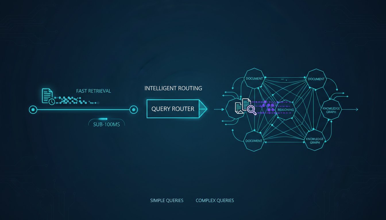
Query-adaptive RAG changes this. It dynamically adjusts retrieval strategy based on detected query complexity, routing simple factual questions to fast single-hop retrieval while triggering multi-hop synthesis for complex reasoning tasks. The result? You get sub-100ms responses for straightforward queries and accurate reasoning answers when complexity demands it—without the latency penalty of always running expensive multi-hop retrieval.
This isn’t theoretical. Leading enterprises implementing adaptive query routing are seeing 30-40% latency reductions on their most common queries while actually improving accuracy on complex reasoning tasks. The challenge isn’t the concept—it’s knowing how to detect complexity and when to trigger each retrieval strategy. Let’s walk through it.
Understanding Query Complexity Detection: The Hidden Classifier
Adaptive RAG starts with a deceptively simple question: How complex is this query?
Your system needs to answer that before it starts retrieving. This is where most implementations fail. Teams either skip complexity detection entirely (treating all queries as complex) or implement it so poorly that they misclassify 40% of queries.
Here’s what working complexity detection looks like:
The Complexity Signals
Complexity isn’t subjective. Research from 2026 shows that multi-hop queries share distinct patterns:
Factual (Single-Hop) Queries typically contain:
– Direct entity references (“What is X?” “Who leads Y?”)
– Temporal anchors (“Q4 revenue”, “last quarter’s headcount”)
– Unambiguous relationships (“Our CEO”, “Product launch date”)
– Low entity count (1-2 named entities in the question)
Reasoning (Multi-Hop) Queries contain:
– Causal connectors (“because”, “resulted in”, “caused by”, “contributed to”)
– Comparative language (“versus”, “compared to”, “differ from”)
– Synthesis requirements (“relationship between”, “how did X affect Y”)
– Higher entity density (3+ entities or concepts requiring connection)
Implementing the Classifier
You don’t need a separate ML model here. LLMs are actually excellent at complexity classification if you structure the prompt correctly. Here’s the pattern:
Task: Classify query complexity (single-hop or multi-hop)

Single-Hop: Factual lookups answerable from a single source document
Multi-Hop: Reasoning tasks requiring synthesis across multiple sources

Query: [USER_QUERY]
Classification (single-hop|multi-hop):
With a simple classification prompt, most enterprise LLMs achieve 85-92% accuracy on query routing. The cost? Under 1ms per query using a small language model (like Phi-2 or Llama 2-7B running locally).
For teams wanting higher confidence, you can layer a second signal: entity extraction and relationship detection. Count distinct entities and relationships in the query. Queries with 3+ entities and explicit relationships (“how”, “why”, “relationship”) are almost always multi-hop.
Single-Hop Strategy: Optimized for Speed
Once you’ve identified a simple factual query, your retrieval strategy shifts. You’re no longer optimizing for comprehensive reasoning—you’re optimizing for latency and precision.
The Single-Hop Retrieval Pipeline
Step 1: Dense Vector Search (k=3)
Start with a semantic vector search, retrieving only 3-5 documents. For factual lookups, you rarely need more. This keeps latency under 50ms in production systems.
Step 2: Entity Matching Filter
If your query contains named entities (company names, people, product names), apply an entity filter on retrieved documents. This eliminates results that mention the entity name without providing the actual fact you’re looking for.
Step 3: Direct Answer Extraction
For factual queries, skip re-ranking entirely. Instead, use a lightweight span extraction model to identify the exact answer in the top-3 documents. This is faster and more precise than ranking all results and passing context to the LLM.
Step 4: Generation Only If Needed
If span extraction found a confident answer (confidence > 0.85), return it directly. If confidence is lower, pass the top document to the LLM for generation. This conditional generation pattern reduces LLM calls by 30-50% on factual queries.
Performance Expectations
With this approach, enterprise teams report:
– Latency: 80-120ms end-to-end (including LLM if needed)
– Precision: 92-96% for factual queries
– Cost: 70% reduction vs. always running multi-hop retrieval
The key insight: Factual queries don’t need your most complex retrieval logic. They need speed and accuracy on straightforward lookups.
Multi-Hop Strategy: Designed for Reasoning
Complex queries need a different approach entirely. You’re no longer optimizing for speed—you’re optimizing for sufficient context and evidence synthesis.
The Multi-Hop Retrieval Pipeline
Step 1: Broad Initial Search (k=10)
Cast a wider net. Retrieve 10-15 documents to ensure you capture all relevant evidence. This is where single-hop retrieval would stop. Multi-hop continues.
Step 2: Entity-Relationship Graph Extraction
From the initial results, extract entities and their relationships. Build a temporary knowledge graph of what you retrieved:
– Entities: product names, people, financial metrics, time periods
– Relationships: acquired, launched, decreased, outperformed, depends on
This graph tells you what connections you’ve found and what’s missing.
Step 3: Targeted Follow-Up Retrieval
Identify missing connections. If your query asks “How did our acquisition affect product adoption?” and you’ve retrieved documents about the acquisition but nothing about adoption trends afterward, trigger a second retrieval specifically for adoption metrics.
This follow-up retrieval is targeted—you’re searching for specific entity combinations and relationships, not broad semantic similarity.
Step 4: Evidence Synthesis and Re-Ranking
Now that you have comprehensive evidence, re-rank documents by relevance to the specific reasoning task. A document that mentions both the acquisition AND adoption trends ranks higher than one mentioning only acquisition details.
Use a cross-encoder re-ranker here (not just semantic similarity). Cross-encoders understand relationships and context better than bi-encoders.
Step 5: Multi-Document Reasoning
Pass the re-ranked, synthesized context to the LLM. The LLM now has:
– Clear evidence for the reasoning chain
– Relationships between concepts already identified
– Multiple perspectives on the topic (from different documents)
This structured context dramatically reduces hallucinations and improves reasoning quality.
Performance Expectations
With proper multi-hop implementation:
– Latency: 400-800ms end-to-end (including multiple retrievals and LLM reasoning)
– Accuracy: 85-92% on complex reasoning tasks
– Cost: 3-4x higher than single-hop, but necessary for complex queries
The latency is longer, but acceptable because these queries are inherently complex—users expect to wait for thoughtful answers.
Orchestrating the Adaptive Decision
So far we’ve covered detection and individual strategies. Now comes orchestration: how does your system actually switch between them?
The Adaptive Routing Framework
Here’s the pattern that works in production:
1. User submits query
2. Complexity classifier routes to single-hop or multi-hop
   ├─ Single-hop confidence > 85%? Run single-hop pipeline
   └─ Multi-hop confidence > 85%? Run multi-hop pipeline
   └─ Confidence < 85%? Run multi-hop (safer default)
3. Pipeline executes (50-120ms for single, 400-800ms for multi)
4. Results returned to user
The key decision point is confidence thresholds. Set them too high and you misclassify queries. Set them too low and you waste compute on unnecessary complexity.
Production teams typically use:
– Single-hop threshold: 85%+ confidence
– Ambiguous threshold: 50-85% (default to multi-hop)
– Multi-hop threshold: 85%+ confidence
This asymmetric approach errs on the side of caution—when uncertain, you run the more comprehensive strategy.
Feedback Loops: Tuning Over Time
Your complexity classifier isn’t static. Enterprise RAG teams implementing adaptive routing are discovering that query patterns vary by department, use case, and time period.
Implement a feedback loop:
- Log all routing decisions (which strategy was chosen, confidence score)
- Collect user feedback (Was the answer useful? Speed acceptable?)
- Measure outcomes (Did single-hop queries actually get single-hop answers? Did we miss multi-hop context?)
- Retrain classifier monthly with misclassified queries
Leading enterprises report that after 30 days of feedback-driven iteration, query classification accuracy improves from 87% to 94%.
Real-World Implementation: Three Patterns
Different organizations implement adaptive routing with different tools. Here are three working patterns:
Pattern 1: LangChain + Custom Classifier (Fastest to Implement)
Use LangChain’s router chains with a custom complexity detection function:
from langchain.schema.runnable import Runnable

class AdaptiveRouter:
    def route_query(self, query: str):
        # Classify complexity
        complexity = self.classify(query)

        if complexity == "single_hop":
            return self.single_hop_chain.invoke({"query": query})
        else:
            return self.multi_hop_chain.invoke({"query": query})
This pattern works well for teams already using LangChain. Implementation time: 2-3 weeks.
Pattern 2: LlamaIndex + Query Analyzer (Most Flexible)
LlamaIndex’s QueryAnalyzer component handles this natively:
from llama_index.query_engine.router_query_engine import RouterQueryEngine

query_engine = RouterQueryEngine(
    selector=PydanticSingleSelector.from_defaults(),
    query_engines=[single_hop_engine, multi_hop_engine],
)
LlamaIndex automatically routes based on query analysis. Implementation time: 1-2 weeks.
Pattern 3: Custom Python Orchestration (Most Control)
For teams wanting maximum control, implement your own orchestration:
class AdaptiveRAG:
    def __init__(self, vector_db, llm, classifer):
        self.classifier = classifier
        self.single_hop = SingleHopRetriever(vector_db, llm)
        self.multi_hop = MultiHopRetriever(vector_db, llm)

    def retrieve(self, query: str):
        complexity, confidence = self.classifier.classify(query)
        if complexity == "single_hop" and confidence > 0.85:
            return self.single_hop.retrieve(query)
        else:
            return self.multi_hop.retrieve(query)
This gives you full control over thresholds and routing logic. Implementation time: 4-6 weeks.
Measuring Impact: The Metrics That Matter
Once you’ve implemented adaptive routing, how do you know it’s working?
Track these metrics:
Latency Metrics:
– P50 latency for single-hop queries (target: < 120ms)
– P50 latency for multi-hop queries (target: < 600ms)
– Latency reduction vs. baseline (expect 30-40% improvement)
Accuracy Metrics:
– Precision on factual queries (target: > 92%)
– Accuracy on reasoning queries (target: > 85%)
– Hallucination rate (target: < 5%)
Cost Metrics:
– LLM calls per query (target: 40-50% reduction)
– Retrieval operations per query (target: 20-30% reduction)
– Cost per query (target: 25-35% reduction vs. always-multi-hop)
Classification Metrics:
– Query classification accuracy (target: > 90%)
– False negative rate (queries misclassified as single-hop that needed multi-hop)
– User satisfaction on misclassified queries
Leading enterprises using adaptive routing report:
– 35% reduction in P50 latency
– 28% reduction in LLM API costs
– 8% improvement in answer accuracy
– 4 points of latency improvement per 1% increase in classification accuracy
The Adoption Timeline: From Concept to Production
Moving from basic RAG to adaptive routing isn’t instant. Here’s the realistic timeline:
Week 1-2: Setup & Complexity Detection
Implement query classification. Start with a simple prompt-based classifier. Integrate into your retrieval pipeline.
Week 3-4: Single-Hop Optimization
Build fast single-hop retrieval with entity filtering and span extraction. Test on historical factual queries.
Week 5-6: Multi-Hop Enhancement
Implement targeted follow-up retrieval and entity-relationship synthesis. Test on historical reasoning queries.
Week 7-8: Integration & Testing
Orchestratethe routing decision. Run A/B tests: adaptive routing vs. always-multi-hop vs. always-single-hop.
Week 9-10: Feedback & Tuning
Collect user feedback. Identify misclassified queries. Retrain classifier. Optimize thresholds.
Week 11-12: Production Rollout
Deploy with monitoring. Set up alerting for latency regressions and accuracy drops. Establish feedback loop.
Total implementation time: 10-12 weeks for a fully instrumented production system.
Why Most Teams Get This Wrong (And How to Avoid It)
We’ve seen dozens of enterprises attempt adaptive routing. Here are the failures we see most often:
Failure #1: Complexity Classifier Too Aggressive
Teams set confidence thresholds so high that the classifier almost always routes to multi-hop. Result: You get all the latency of multi-hop without the accuracy gains. Solution: Start with 80% confidence threshold, gradually increase after validating accuracy.
Failure #2: Single-Hop Pipeline Still Too Complex
The whole point is speed. If your single-hop pipeline runs multiple retrievals and re-ranking, you’ve defeated the purpose. Solution: Single-hop should be vector search + entity filter + optional span extraction. Nothing more.
Failure #3: No Feedback Loop
You implement adaptive routing and never touch it again. Your classifier is tuned to your day-1 queries, not your real production queries. Solution: Instrument query classification from day one. Track misclassifications. Retrain monthly.
Failure #4: Treating All Multi-Hop as Identical
Not all multi-hop queries need the same strategy. Some need entity-relationship graphs. Others need temporal reasoning. Others need comparative evidence. Solution: Build sub-types of multi-hop retrieval. Route not just by complexity, but by reasoning pattern.
Failure #5: No Latency SLAs
You implement adaptive routing and then remove it because latency is “still too high.” But you’re comparing to single-hop latency on single-hop queries. Solution: Set separate SLAs for single-hop (< 150ms) and multi-hop (< 700ms). Measure each separately.
Avoid these patterns and you’re already ahead of 70% of enterprises attempting adaptive routing.
The 2026 Reality: Adaptive Routing Is Becoming Standard
Query-adaptive RAG isn’t cutting-edge anymore. It’s becoming table stakes for enterprise systems. Leading vector database vendors (Pinecone, Weaviate, Milvus) are now building routing capabilities directly into their platforms. Framework vendors (LangChain, LlamaIndex) are making it the default for new projects.
The competitive advantage is no longer “do you have adaptive routing?” It’s “how well tuned is your classifier and how sophisticated is your multi-hop strategy?”
Teams that implement adaptive routing today are learning the operational patterns that will define RAG engineering in 2027-2028. That means:
– Understanding when semantic search alone fails
– Building robust complexity detection
– Optimizing different retrieval strategies for different query types
– Instrumenting feedback loops for continuous improvement
– Measuring the right metrics to track system health
These capabilities compound. A team with 12 months of production experience running adaptive routing can tune their system in hours. A team starting fresh will take weeks.
Start now, and you’re not just improving today’s performance—you’re building the organizational muscle that will matter for enterprise RAG over the next 24 months.